10 Mar 2017
In this blog post we describe how to view DINAMITE traces using
TimeSquared.
In the previous post we
described how to query DINAMITE traces using a SQL database.
If you would like to get an idea of what the output of TimeSquared will look
like, check out the
demo. Just
click on any button under ‘Sample Data’.
Pre-requisite: You will need to set up the database as described in that
post and try the example queries, because TimeSquared interfaces with the
database to show portions of the trace.
Set up TimeSquared:
   # Clone the repository
   % git clone https://github.com/dinamite-toolkit/timesquared.git
   % cd timesquared

   # Install all dependent modules
   % npm install
   % npm install monetdb

   # Start the server
   % cd timesquared/timesquared
   % node server.js
If you are using the settings for MonetDB other than the ones recommended in
our previous post, modify
timesquared/server/TimeSquaredDB.js to reflect these changes. The default
options look like these:
   var MDB_OPTIONS = {
   host : 'localhost',
   port : 50000,
   dbname : 'dinamite',
   user : 'monetdb',
   password : 'monetdb'
   };
As you can see, they reflect the same database name, user name and password, we
used for MonetDB.
If your server ran successfully, you will see a message like this:
TimeSquared server hosted on http://:::3000
Open your browser and type the following for the URL:
Click on the "Dashboard" button. You will see a textbox, where you can begin
typing SQL queries to visualize parts of the trace.

Suppose that after reading the [previous
post](/2017/03/10/querying-dinamite-traces) you want to generate a portion to
the trace corresponding to the time when a function of interest took a
particularly long time to run. Suppose that you found, using the query `SELECT *
FROM outliers ORDER BY duration DESC;` that the ID of your "outlier" function
invocation equals to 4096.

Type the following query into the query box and press the "Query" button.
with lbt as (select time from trace where id=4096 and dir=0), ubt as
(select time from trace where id=4096 and dir=1) select dir, func, tid, time
from trace where time>= (select time from lbt) and time<=(select time from
ubt)
```
The browser will open another tab where it will try to render the results of
your query. You can watch the console where you started the server for any log
messages indicating the progress, or error messages. If there are too many
records in the result of your query (e.g., >500K), the rendering will take a
long time and may even crash the browser. In that case, try limiting the number
of records returned by adding the ‘LIMIT’ command to the end of the query. For
instance, to limit the results to 100,000 records, append ‘LIMIT 100000’ to the
query above.
Once rendering is complete, you will see a succession of callstacks
over time, for each thread. Time flows on the horizontal axis, threads
and callstacks are along the vertical axis, like so:
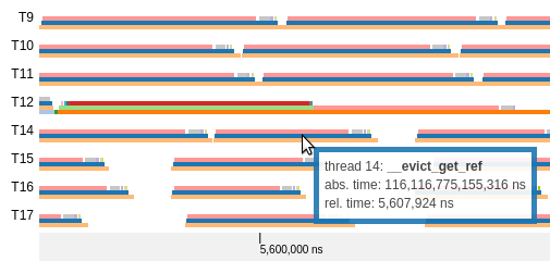
If you hover with the mouse over a coloured strip in the callstack,
TimeSquared will show you the name of the function and some
information about it.
If you want to see what the TimeSquared output will look like you can
TimeSquared is work in progress. We are working on building an interface to
effectively navigate very large traces. At the moment TimeSquared cannot show
too many events – and even if it could, you’d hardly want to look at all of
them. We will report on these features in our future blog posts.
10 Mar 2017
In this blog post we describe how to query DINAMITE traces using SQL.
Setting up the database and importing traces
If you have read our earlier
post,
you know how to process the binary trace files generated by DINAMITE
using the process-logs.py script.
This script will produce a compressed trace.sql.gz file with the entire trace
in a human-readable format, and a few SQL commands allowing you to import this
file directly into the database. That way, you can query your trace using the
mighty SQL!
If for some reason you don’t want to use a database, you can visually examine
the trace.sql file and query it using any other tools you like, because it is
just plain text (just remove the SQL commands at the top and at the bottom of
the file). In that case, decompress the file first by running gunzip
trace.sql.gz.
If you are a brave soul willing to embrace the power of databases, we will tell
you how to set up a free database MonetDB and use it to query the trace.
-
Download and install MonetDB as explained here.
- Start the database daemon and create the database called ‘dinamite’ like so:
monetdbd create monetdb
monetdbd start monetdb
monetdb create dinamite
monetdb release dinamite
-
Create a file .monetdb in your home directory with the following
content. This is needed, so you don’t have to type the username and
password every time. Note, we are using the default password for the
trace database. If you want to protect your trace with a stronger
password, change it accordingly and don’t put it in the text file.
user=monetdb
password=monetdb
-
Import the trace.sql.gz file created by process-logs.py into the database:
gunzip -c trace.sql.gz | mclient -d dinamite
You are good to go! Now you can query your traces using SQL. For those
not fluent in SQL we provide a few example queries to get you started.
Querying the traces
The database you created in the preceding steps will have three
tables: trace,avg_stdev and outliers. The trace table contains
raw trace records sorted by time. The avg_stdev table contains the
average duration and the standard deviation of durations for each
function. The table outliers contains the functions whose duration
was more than two standard deviations above the average.
The tables have the following schema:
   CREATE TABLE "sys"."trace" (
    "id"       INTEGER,
    "dir"      INTEGER,
    "func"     VARCHAR(255),
    "tid"      INTEGER,
    "time"     BIGINT,
    "duration" BIGINT
   );
where id is the unique identifier for each invocation of a function,
dir is an indicator whether the given record is a function entry
(dir=0) or exit point (dir=1), func is the function name, tid is
the thread id, time is the timestamp (in nanoseconds, by default),
and duration is the duration of the corresponding function.
   CREATE TABLE "sys"."avg_stdev" (
    "func"  VARCHAR(255),
    "stdev" DOUBLE,
    "avg"   DOUBLE
   );
where func is the function name, avg is its average duration
across all threads and stdev is the standard deviation.
   CREATE TABLE "sys"."outliers" (
    "id"       INTEGER,
    "func"     VARCHAR(255),
    "time"     BIGINT,
    "duration" BIGINT
   );
where id is the unique ID for each function invocation, func is
the function name, time is the timestamp of the function’s entry
record and duration is the duration.
You can examine the schema yourself by opening a shell into the
database, like so:
and issuing a command ‘\d’. Running this command without arguments
will list all database tables. Running this command with a “table”
argument will give you the table’s schema, for example:
Suppose now you wanted to list all “outlier” functions, sorted by
duration. You could accomplish this by typing the following SQL query:
sql> SELECT * FROM outliers ORDER BY duration DESC;
Or if you wanted to display the first 10 entry records for functions that took
more than 60 milliseconds to run:
sql> SELECT * FROM trace WHERE duration > 60000000 AND dir=0 LIMIT 10;
Now, suppose you wanted to see what happened during the execution
while an particular unusually long function was running? You could list all
events between the boundaries of the outlier function, sorted in the
chronological order, via the following steps.
-
First, find the ID of the outlier function invocation you want
to examine using the SELECT * FROM outliers ORDER BY duration
DESC;, picking any function you like and noting its ID (the first
column). Suppose you picked a function invocation with the id 4096.
-
Run the following query to obtain all concurrent events:
   sql> WITH lowerboundtime AS
   (SELECT time FROM trace WHERE id=4096 AND dir=0),
   upperboundtime AS
   (SELECT time FROM trace WHERE id=4096 and dir=1)
   SELECT * FROM trace WHERE
   time>= (SELECT * FROM lowerboundtime)
   AND time <= (SELECT * FROM upperboundtime);
That query will probably give you a very large list of events – so
large that it’s really inconvenient to look at it in a text form. To
make viewing event traces more pleasant, we built a tool called
TimeSquared. You can use it to view event traces generated from SQL
queries. Read about it in our next blog
post!
And before we finish this post, here is another very useful query that
could help diagnose the root cause of an “outlier” function
invocation. The following query will list all the children
function-invocations of the long-lasting functions and sort them by
duration. This way, you can quickly spot if there is a particular
callee that is responsible for high latency in the parent. Again,
assuming that you previously determined that the id of the
long-lasting function equals to 4096 and the function was executed by
the thread with tid=18, the query would look like:
   sql> WITH lowerboundtime AS
   (SELECT time FROM trace WHERE id=4096 AND dir=0),
   upperboundtime AS
   (SELECT time FROM trace WHERE id=4096 and dir=1)
   SELECT func, id, time, duration FROM trace WHERE
   time>= (SELECT * FROM lowerboundtime)
   AND time <= (SELECT * FROM upperboundtime)
   AND tid=18  ORDER BY	duration DESC;
06 Mar 2017
In this blog post we describe how we use DINAMITE to compiled RocksDB, an open
source persistent key-value store developed by Facebook.
Building RocksDB
Here is the RocksDB Github Repo of
RocksDB. If you have your gcc correctly set up, a
simple make static_lib db_bench instruction in the root of the repo can build a ‘‘normal’’ version of RocksDB static library and some db_bench sample applications.
Build and Run With Docker
-
A Docker container with LLVM and DINAMITE can be found here. Run and setup the docker as suggested in the repo.
-
In the docker command line, setting the following environment variables:
export WORKING_DIR=/root/dinamite
export LLVM_SOURCE=$WORKING_DIR/llvm-3.5.0.src
export LLVM_BUILD=$WORKING_DIR/build
-
Clone the RocksDB.
cd $WORKING_DIR
git clone https://github.com/facebook/rocksdb.git
cd rocksdb
-
Set up environment variables for building RocksDB with DINAMITE
# Variables for DINAMITE build:
export PATH="$LLVM_BUILD/bin:$PATH"
export DIN_FILTERS="$LLVM_SOURCE/projects/dinamite/function_filter.json" # default filter
export DIN_MAPS="$WORKING_DIR/din_maps"
export ALLOC_IN="$LLVM_SOURCE/projects/dinamite"
export INST_LIB="$LLVM_SOURCE/projects/dinamite/library"

# variables for loading DINAMITE pass on RocksDB:
export CXX=clang++
export EXTRA_CFLAGS="-O3 -g -v -Xclang -load -Xclang $LLVM_SOURCE/Release+Asserts/lib/AccessInstrument.so"
export EXTRA_CXXFLAGS=$EXTRA_CFLAGS
export EXTRA_LDFLAGS="-L$LLVM_SOURCE/projects/dinamite/library/ -linstrumentation"

# Set up variables for runtime, can be set up later before running
export DINAMITE_TRACE_PREFIX=$WORKING_DIR/din_traces
export LD_LIBRARY_PATH=$INST_LIB

# Create directories if not exist:
mkdir $DIN_MAPS
mkdir $DINAMITE_TRACE_PREFIX
Note: If you are running on MacOS, please do the following changes:
export EXTRA_CFLAGS="-O3 -g -v -Xclang -load -Xclang $LLVM_SOURCE/Release+Asserts/lib/AccessInstrument.dylib"
export DYLD_LIBRARY_PATH=$INST_LIB
-
Build the RocksDB library and some sample applications.
make clean
make static_lib db_bench
cd examples
make clean
make
cd ..
-
Now run the simple example RocksDB program to get some traces!
cd examples
./simple_example
Build and Run in Your Own Environment
If you don’t like docker (don’t worry, we have the same feeling), you can definitely build DINAMITE instrumented RocksDB in your own environment.
-
Basically you need to (1) build your LLVM; (2) Place DINAMITE pass to the correct place; (3) Build DINAMITE pass and its runtime library.
You can copy the commands in the Dockerfile to apply them appropriately to your system. Details information is provided in the section Environment in another article Compiling the WiredTiger key-value store using DINAMITE.
-
Make sure your are assigning those environment variables correctly:
export WORKING_DIR="Your working directory, which will later contain rocksdb repo"
export LLVM_SOURCE="Your LLVM source base directory"
export LLVM_BUILD="The directory contains your LLVM build. This directory is supposed to have a directory called bin, which contains the clang/clang++ binary"
-
Do the same things starting from (including) Step 3 in section Build and Run With Docker.
Appendix
DINAMITE Variables Explanation:
* `DIN_FILTERS` is a configuration file in json format indicating what get filtered out for injecting instrumentation code
* `DIN_MAPS` is the place where storing id to name maps, important for processing later traces.
* `ALLOC_IN` is a directory contains alloc.in, which let you specify your allocation function
* `INST_LIB` is the variable telling the runtime library DINAMITE uses for writing traces
If you run into trouble, get in touch. If you’d like to find out how to control what’s instrumented, take a look at the
User Guide. If you’d like to know what to do with the traces now that you have them,
take a look at the other Technical Articles
03 Feb 2017
This post describes how we discovered a source of scaling problems for
the multireadrandom benchmark in RocksDB.
A while ago, we ran some scaling tests on a set of RocksDB benchmarks. We
noticed that some of the benchmarks didn’t scale well as we increased the number
of threads. We decided to instrument the runs and use
FlowViz to visualize
what is going on with multithreaded performance. The discovery helped open two
issues in RocksDB’s repository:
1809 and
1811.
Here’s what we did:
(This tutorial was tested on DINAMITE’s docker
container. To set
it up, follow our Quick start guide. If any of the instructions
do not work in your environment, please contact us.)
Setting up RocksDB
Configuring RocksDB to use DINAMITE’s compiler is straightforward.
The following is a set of environment variables that need to be set in order to
do this. Save it into a file, adjust the paths to point to your DINAMITE
installation path, and source before running ./configure
############################################################
## source this file before building RocksDB with DINAMITE ##
############################################################

export DIN_FILTERS=/dinamite_workspace/rocksdb/rocksdb_filters.json
export DINAMITE_TRACE_PREFIX=<path_to_trace_output_dir>
export DIN_MAPS=<path_to_json_maps_output_dir>
export EXTRA_CFLAGS="-O0 -g -v -Xclang -load -Xclang
${LLVM_SOURCE}/Release+Asserts/lib/AccessInstrument.so"
export EXTRA_CXXFLAGS=$EXTRA_CFLAGS
export EXTRA_LDFLAGS="-L${INST_LIB} -linstrumentation"
Make sure that $LLVM_SOURCE points to the root of your LLVM build, and that
$INST_LIB points to the library/ subdirectory of DINAMITE compiler’s root.
The contents of rocksdb_filters.json are as follows:
{
    "blacklist" : {
        "function_filters" : [
            "*atomic*",
            "*SpinMutex*"
        ],
        "file_filters" : [ ]
        },
    "whitelist": {
        "file_filters" : [ ],
        "function_filters" : {
            "*" : {
                "events" : [ "function" ]
            },
            "*SpinMutex*" : {
                "events" : [ "function" ]
            },
            "*InstrumentedMutex*" : {
                "events" : [ "function" ]
            }
        }
    }
}
Run ./configure in RocksDB root, and then run make release.
After the build is done, you should have a db_bench executable in RocksDB
root.
Running the instrumented benchmark
The following is the script we used to obtain our results:
#!/bin/bash
BENCH=$1
THREADS=$2
./db_bench --db=<path_to_your_db_storage> --num_levels=6 --key_size=20 --prefix_size=20 --keys_per_prefix=0 --value_size=100 --cache_size=17179869184 --cache_numshardbits=6 --compression_type=none --compression_ratio=1 --min_level_to_compress=-1 --disable_seek_compaction=1 --hard_rate_limit=2 --write_buffer_size=134217728 --max_write_buffer_number=2 --level0_file_num_compaction_trigger=8 --target_file_size_base=134217728 --max_bytes_for_level_base=1073741824 --disable_wal=0 --wal_dir=/tmpfs/rocksdb/wal --sync=0 --disable_data_sync=1 --verify_checksum=1 --delete_obsolete_files_period_micros=314572800 --max_background_compactions=4 --max_background_flushes=0 --level0_slowdown_writes_trigger=16 --level0_stop_writes_trigger=24 --statistics=0 --stats_per_interval=0 --stats_interval=1048576 --histogram=0 --use_plain_table=1 --open_files=-1 --mmap_read=1 --mmap_write=0 --memtablerep=prefix_hash --bloom_bits=10 --bloom_locality=1 --benchmarks=${BENCH} --use_existing_db=1 --num=524880 --threads=${THREADS}
Make sure you fix the --db argument to point to where your database will be
stored. In our case, the first argument ($BENCH) was set to multireadrandom
and the number of threads varied from 1 to 8 in powers of 2.
Results
The output logs were processed and visualized with FlowViz. The guide on how to
use this tool is available here
and will be omitted from this post for brevity.
Here is the FlowViz output for runs with 1 and 8 threads:
1 thread:
8 threads:
From these, it is immediately obvious that the amount of time spent performing
locking operations increases with the number of threads.
These results were used to infer inefficiencies in workloads using MultiGet()
and led to opening of the two aforementioned issues on the RocksDB tracker.
20 Dec 2016
In this post we introduce DINAMITE’s execution flow charts – charts
that visually convey both how the program works and how it performs.
Our previous post
described how to parse binary traces created in the process of running the
DINAMITE-instrumented program. The parsing step will convert the binary traces to
text, create summary files, and generate execution flow charts showing how the
program transitions between different functions and how much time
it spends there.
The process-logs.py script in the binary trace toolkit (see
previous
post)
will now produce a directory called HTML in the same directory where
you ran the script. By opening HTML/index.html inside your browser,
you will see execution flow charts for all threads on a single page
and clicking on any image takes you to a new page, where this image is
interactive: you can click on rectangles corresponding to different
functions to get summaries of their execution. Let us go through all
of this in more detail.
First, let’s take another look at an execution flow chart. The one below is for
one of the application threads in a a multi-table workload executing on top of
the WiredTiger key-value store.
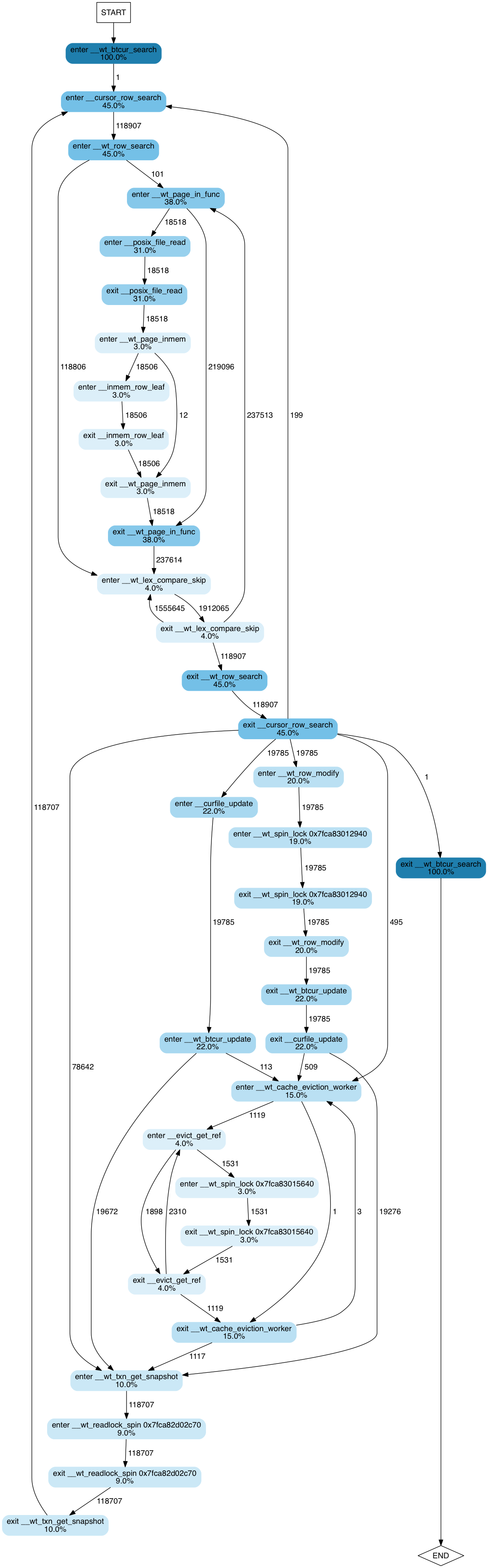
The image shows a state transition diagram, where states are function
entry/exit points. Edges between states show how many times each
transition occurs. Nodes corresponding to states are coloured and
annotated accordingly to percent of execution time spent by this
thread in the corresponding function. Percent values are
cumulative. That is, if foo() took 100% of the execution, and bar(),
called by foo(), took 90%, they will be annotated as 100% and 90%
respectively.
From this diagram we can intuit how the program works, even if we have
never seen the code and have only a vague understanding of how
key-value stores work. We observe that it searches a btree (100% of
the time is spent in __wt_btcur_search), which probably has a
row-based layout (__wt_row_search, __cursor_row+search). We can
guess that in this execution the thread performed 118,907 searches
(the number of transitions between enter __cursor_row_search and
enter __wt_row_search) and of those searches most of the records
(118,806, to be precise) were found in memory: we can guess the latter
from the fact that there are 118,806 transitions directly from enter
__wt_row_search to enter __wt_lex_compare_skip. 110 of the
searches, on the other hand, did not find the needed page in memory
and caused the system to read the data from disk: hence the right
subtree emanating from the enter __wt_row_search function and
dominated by __wt_page_in_func (38% of the execution time) – the
function that, judging by its name, pages the data from disk.
Furthermore, we get interesting statistics about the effect of locks on performance.
- ~19% of the time is spent waiting on a spinlock somewhere in
__wt_row_modify function (or its children).
- A lock acquired by
__evict_get_ref takes about 3% of the execution time
- There is also a read/write spinlock, acquired by
__wt_txn_get_snapshot (or
its children) — it takes about 9% of the execution time for this thread.
Note that lock releases are not shown here, because they take less than 2% of
the execution time, and by default the trace-processing script filters any
functions with small contributions to the overall time to avoid having to show
a huge number of nodes.
Now, if you follow this
link, you will
be taken to a page that includes interactive version of execution flow
charts for all threads for the same workload.
If you click on any image, you will be taken to a page where the same image is
interactive. You can click on any node of the flow diagram and be taken to a
page containing a short summary of this function’s execution. Those summaries are
not great yet; we are working on making them more useful, but one curious thing
we discover from them, by clicking on a summary for any lock-acquiring function,
is that the largest time to acquire a lock was more than a whole second (!!!) –
much larger than the average time to acquire the lock. This is definitely a red
flag that a performance engineer would want to investigate.
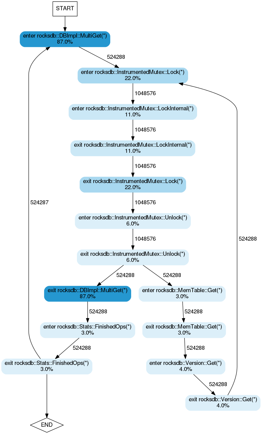
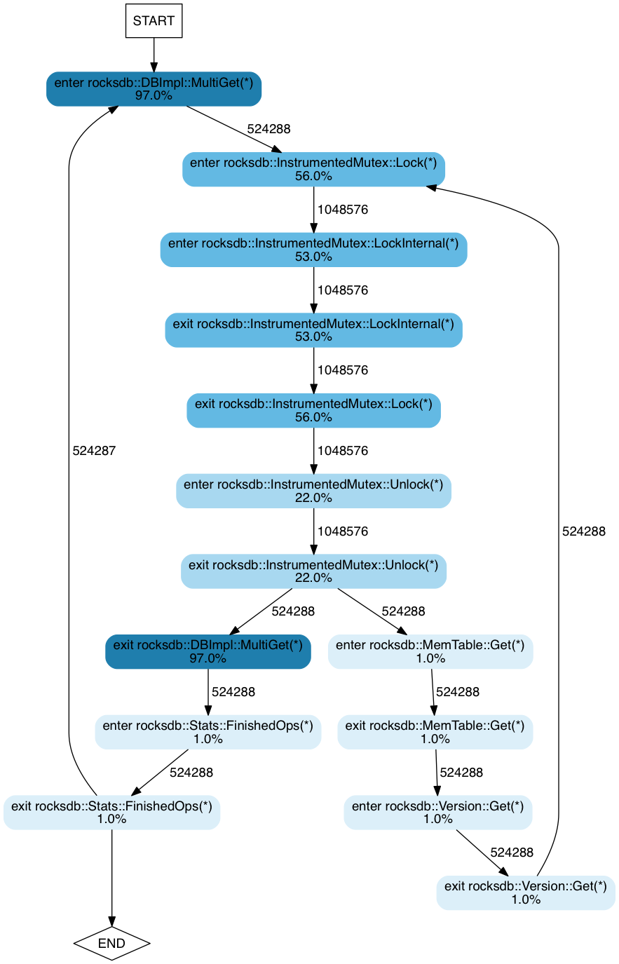
For another example, take a look at the following execution flow
charts for RocksDB. We executed dbbench with the multireadrandom
workload using
one,
two,
four
and
eight
threads respectively. Note how the time spent acquiring locks
increases as we increase the number of threads.
Note: If you have already converted binary traces to text and want to
re-generate the HTML, simply go into the directory containing text traces
and run:
% $DINAMITE_BINTRACE_TOOLKIT/process_logs.py trace.bin.*.txt
By default, all functions taking less than 2% of the execution time
will not be included in the diagrams. To remove this filter, run the
script like this:
% $DINAMITE_BINTRACE_TOOLKIT/process_logs.py -p 0.0
   trace.bin.*.txt
The -p argument controls the percent value for the filter. Without
filtering, the diagrams may become very large and not suitable for
viewing.
See previous post
if you need information on how to download the DINAMITE binary trace toolkit.